Subjects
Two male subjects (authors MS & SK) were scanned extensively for this project. Both subjects were healthy controls with no history of neurological conditions. Subject 1 was 47 years and Subject 2 was 30 years at the time of the scanning.
Scanning Acquisition Parameters
T1w, T2w, and Proton Density (PD) images were acquired on a Siemens 7T MAGNETOM at the Centre for Advanced Imaging using a 32-channel head coil. Diffusion Weighted Imaging (DWI) data were acquired at on a Philips 3T Ingenia CX at the NeuRA Imaging Centre using a 32-channel head coil.
T1w: MP2RAGE sequence (WIP944). Three different T1w protocols were used: Dutch, Flaws, & MP2RAGE. Dutch Protocol parameters: Voxel size=0.5mm3,TR=6000ms, TE=3.18ms, TI1=1200ms, TI2=4790ms, GRAPPA=3. Flaws Protocol parameters: Voxel size=0.6mm3,TR=5000ms, TE=1.49ms, TI1=620ms, TI2=1450ms, GRAPPA=3. MP2RAGE Protocol parameters: TR=4300ms, TE=1.8ms, TI1=830ms, TI2=380ms, GRAPPA=2. T2w: TSE sequence (WIP692) at 0.4 mm3 isotropic resolution with the parameters: TR=1330ms, TE=118ms, GRAPPA 3.
Proton Density (PD): Protocol parameters: Voxel Size = 1.0mm3, TR=6.0ms, TE=3.0ms, GRAPPA=2 •One PD scan was collected during each scanning session in order to correct for luminance inhomogeneities present in our T1w scans (Van de Moortele et al, 2009). This is described in more detail in the Data Analysis section.
Data Analysis
T1w: Preprocessing: Each T1w scan type (Dutch, Flaws, MP2RAGE) was preprocessed separately. Preprocessing steps included: 1) The ImageMath command from the ANTs toolbox was used to truncate the luminance intensities of each scan with 0 as the lower quantile and 0.999 as the upper quantile. 2) Removing unnecessary parts of the scan (neck, nose, etc) to decrease file size. The robustfov script from FSL was used for this. 3) Upsampling the voxel size to 0.25mm3. This was done in order to ensure voxel sizes were uniform across different scan protocols and modalities, and to also decrease the effect of blurring caused by ‘reslicing’ or applying an alignment transform to an image. 4) Ensuring all the dimensions of each scan was 1024. As in Step 3, this was used in order to ensure uniform dimensions across different scan protocols and modalities. 5) Skull stripping. We conducted this step in order to improve alignment by removing parts of each scan that did not include cortex. We also conducted skull stripping due to the large size of our scans (~1-2Gb), as skull stripping decreased file sizes considerably (~300Mb). For this we used HD-BET to create a brain mask for each scan. While the brain mask provided a good estimate of brain, some brain regions with low signal to noise (e.g. temporal cortex) would not be included in the brain mask and were hence removed during skull stripping. As such, we also created a skull stripped variant with the brain mask inflated by 30mm which would include all brain regions that would be cut out of the original estimate. These files were subsequently used during alignment and averaging. 6) Proton Density Correction. We used the same method proposed by Van de Moortele et al (2009) to correct for luminance inhomogeneities in our T1w images. We did this by aligning a Proton Density image collected during the same scan session for each T1w image, and then divided the T1 image by the aligned Proton Density image. This yielded an image without inhomogeneities, and high grey/white contrast. 7) A linear average was then generated using the files from the previous step. For this the fslmerge command with the –t flag was used in order to create an unbiased linear average that was not influence by the order in which the scans were collected. This linear average was used as a starting point for symmetric group-wise template generation.
T2w: Preprocessing: The scan preprocessing steps conducted for the T1w images were conducted on the T2w images. The only difference was that the T2w images were not proton density corrected.
T1w & T2w: Template generation: Symmetric group-wise normalisation was conducted using Advanced Normalization Tools (ANTs), specifically using the antsMultivariateTemplateConstruction script. The parameters used to align each scan included a Cross Correlation similarity metric (-s flag), a Greedy SyN transformation model used for non-linear registration(-t flag), 20x15x5 was the maximum number of steps in each registration (-m flag), the gradient was 0.1 (-g flag), and the total number of iterations was 4 (-i flag). Each modality (T1w & T2w) was processed separately.
DWI
DWI data was analyzed using MRtrix 3.2 (Tournier et al 2019) and ANT. First each scan was upsampled by a factor of 2×2 in the inplane direction and then preprocessed using the dwifslpreproc script providing topup distortion correction and eddy_cuda correction. Then the preprocessed data was upscaled across slices, again by a factor of 2, so the final output had a resolution of 0.6123 mm3. This upsampling strategy was chosen to increase the spatial detail through averaging repeated acquisitions, however doubling the across slice resolution is incompatible with eddy correction. Hence, across slice resolution was doubled after eddy correction. For each of the 10 upsampled preprocessed DWI datasets a mean DWI image, a FAC (Fractional Anisotropy Color) image as well as a FOD (Fibre Orientation Distribution) using spherical deconvolution through the dwi2fod command using a response function estimate using the dhollander algorithm. Then based on the 10 mean DWI images a mean DWI template [0.5 mm] was constructed using the ANTs software package This transform estimated from the mean DWI images was also applied to the 10 FAC images and 10 ID images using the ANTS software. The ID images then allowed to transform the 10 FOD images into the DWI template space using the mrtranform function from MRtrix which ensured that the FOD vectors were transformed correctly (using the option -reorient_fod yes). FAC images and FOD were then averaged in the DWI template space. This intermediate space was used to save RAM and compute resources where simply averaging 10 FOD images at 0.25mm would require 512GB or RAM). Then all DWI data were transformed into the final ACPC template space (0.25 mm) again using ANTs for the FAC and mean image and ID files and MRtrix for the FOD. Finally, in the ACPC template space of the final atlas, a DEC (Direction Encoded) image was generated using the T1w image for contrasting. fod2dec wmFOD.mif -contrast T1w.nii.gz wmDEC_T1w.mif
Additional Information can be found here: